Last weekend, I enjoyed two webinars by Tim Janzen that were part of MyHeritage’s One-Day Genealogy Seminar with Legacy Family Tree Webinars. Tim gave an introductory talk and an advanced talk on the use of Autosomal DNA Testing.
In both talks, Tim showed the well-known and often referred to Speed and Balding diagram which I’m showing here:
It is also highlighted on the ISOGG Wiki Identical By Descent page, where it says:
“A study by Speed and Balding (2015) using computer simulations going back for 50 generations showed that over 50% of 5 mB segments date back over 20 generations, and fewer than 40% of 10 mB segments are within the last 10 generations. Larger segments can still date back quite some time and it was found that around 40% of 20 mB segments date back beyond 10 generations.”
This analysis is quoted often. It illustrates that small segments are very distant, and even larger segments can be quite distant.
The diagram is from Figure 2B of a paper published online in Nature Reviews Genetics on 18 Nov 2014 by Doug Speed and David J Balding titled “Relatedness in the post-genomic era: is it still useful?” Their entire article has now been made available by Doug Speed at his website. The article is very technical and uses a lot of statistics which will make it impossible for the average person to read. But let it be known that their analysis is well done.
It’s a strange looking chart which demands some explanation. On the X axis are IBD (Identical by Descent) region lengths in Mb. A segment passed down to two people from a common ancestor is IBD. The Mb are million base-pair. 1 Mb is close enough to 1 cM (centimorgan) which approximates the probability of recombination in one generation.
Since recombination occurs each generation, large segments get subdivided. Jim Bartlett gives an excellent example in his Segments: Bottom-Up article. Therefore, segments you get from each ancestor will tend to get shorter the further back you go.
So the Speed and Balding chart is showing ranges of segment length on the X axis and the probability of occurrence on the Y axis. It then stacks the probabilities of each generation having each range of segment length, and color codes each generation. G=1 is shown in red. G=2 to G=9 is shown in alternating dark blue and light blue colors, G=10 is shown in green to highlight that generation, G=11 to G=20 continues with alternating dark blue and light blue colors and G>20 is shown in gray.
Reading the chart, you can make conclusions that for IBD segments between 10 and 20 Mb, only 40% are from an ancestor within 10 generations and 30% are from an ancestor more than 20 generations back. For IBD segments between 5 and 10 MB, only 10% are from an ancestor within 10 generations and 50% are from an ancestor more than 20 generations back.
Incorrect Application of Their Results
This chart is being used by many genetic genealogists to help them conclude that small segments will often yield ancestors that are too far back to be genealogically useful. Matching segments under 5 or 7 cM are often called too small to be of practical use. For endogamous groups, 20 cM or even 30 cM may be called too small.
Speed and Balding’s study was one of descendancy. Their Type B simulation was used for their Figure 2b. They started with 5,000 males and 5,000 females and simulated 50 generations of descendants.
Their simulations are good. Their analysis and statistics are good.
However, their results refer to the final 50th generation of descendants. They calculate the number of generations of IBD each of those people in the final generation have with each other. They state in their paper:
Under the coalescent model, the MRCA of two haploid human genomes at a given site is unlikely to be recent. … In our Type B simulation model, the probability of an MRCA in generation G is … which supports the assumption that people are unrelated if nothing is known about them.
The bottom line is that the Type B simulation data that is summarized for their Figure 2B was including all 6th, 7th, 8th cousins and more and adding their instances to the probability of the instance’s segment length for that particular generation back to the ancestor (G = 7, 8, 9, …)
That is not wrong on their part. But it is wrong to apply their results to our match data from a DNA testing company.
DNA Testing companies screen our matches. They don’t include everyone because they only want to include likely matches. Each company has their own criteria for inclusion. Family Tree DNA for example, will only include a person as a match if they have at least one segment that is 9 cM, or if they have at least one segment that is 7.69 cM and the total shared is greater than 20 cM.
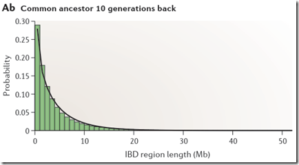
If you take a look at Figure 2Ab in Speed Balding, they show their simulated probability of each region length at 10 generations:
Through inspection, only about 5% of the segments are above 8 or 9 Mb. This implies that only 1 out of 20 people who have a common ancestor at 10 generations back will be identified as a match with you.
Recalculating Speed Balding
We need to apply Speed and Balding’s information, but need to do so for only the people who will show up to you as matches. We need some data to do this.
Unfortunately, Speed and Balding produced Figure 2Ab for 10 generations (shown above), and Figure 2Aa for 1 generation. They do not give the data, but do indicate that the distributions can be approximated by a gamma distribution, which is:
The value of that gives the probability
for x > 0, where x is the IBD region length in Mb.
k is the shape parameter.
Theta is the scale parameter.
In a Gamma distribution, theta can be calculated as the mean / k;
The letter at the bottom left of the equation before “(k)” is the gamma function.
The paper says the shape parameter k is approximately 0.76 for any G.
It says the mean of the distribution is Equation 4, but that is the expected number of IBD segments. The paper should have said Equation 5, which is the mean length of IBD regions which is what is wanted. Equation 5 is:
where G is the number of generations back.
Therefore theta is this mean value divided by k.
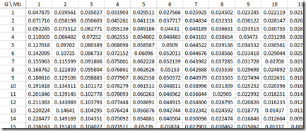
Sorry about all this horrendous maths/stats, but I wanted to show that we now have all the calculations we need to build the approximate probabilities for each IBD region length (Mb) for every G that was used in the paper:
Look at the row where G=10. You’ll see that the values for Mb = 1, 2, 3, … which are 0.191618, 0.134511, … correspond to the black line (gamma distribution estimate) of the green bar chart above for Common Ancestor 10 Generations Back (Speed and Balding Figure 2Ab).
Converting this to Speed and Balding Figure 2B
Now the tricky part.
The paper says it uses a second simulation to get its information for figure 2B. Statistics and the approximate probabilities above should be able to give something close. The clue as to what they are doing is given in their statement that this is the “Inverse Distribution”. i.e. Figure 2A’s distribution is:
Probability(region length) for G = 1, 2, 3, …
They are determining what they are calling the inverse distribution:
Probability(G) for region length = specific ranges
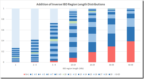
I can group the IBD region length probabilities into the same region lengths as Figure 2B, and I’ll make the following groups: 1 Mb, 2-4 Mb, 5-9 Mb, 10-19 Mb, 20-29 Mb, 30-39 Mb and 40-49 Mb. I can then total the probability of each group for any G and divide that by the total of the column to get the average probability of getting a specific G within a Mb group. Then I can stack those and I get the following:
The numbers are a bit different because (a), theirs is a simulation and not statistics, and (b) the gamma distribution is only an approximation of the simulated distribution, and (c) I only used integer values of IBD region length, whereas their model used real numbers. But this is still reasonably close to the Speed Balding Figure 2B at the top of this post.
This makes me quite confident that the results of their simulation were summarized in a compatible way to give their Figure 2B.
The critical G=10 region shown in green that everyone refers to is a bit higher on the probability model of my estimate, but that difference is well within margins of error and wouldn’t change any conclusions arising from this chart regarding small segment.
Oh Oh.
There’s one critical problem with this analysis. Did you see it?
Their probability distribution values for region length cannot be directly used in an inversion in this manner. The probability distributions of region length are dimensionless. It is a probability that you must first apply to a number of observations. The number of observations you will have for each G is not constant. You have a lot more relatives at G = 6 than you have at G = 1.
Incorporating the Likelihood of IBD DNA being detected.
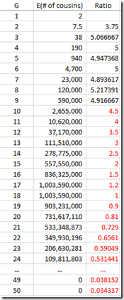
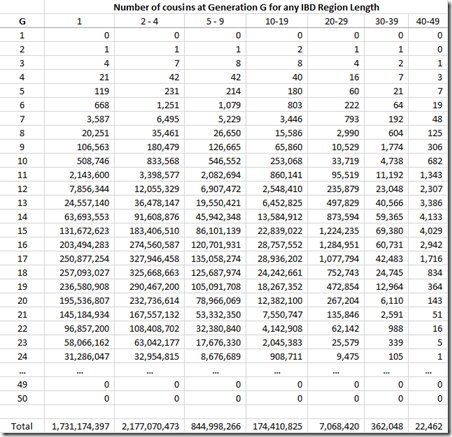
What needs to be done is to multiply each of the probability values by the number of relatives you’ll have at G = 1, 2, … I can get such values from this table on the ISOGG Cousin Statistic page:
I can use the “Expected number of cousins” column and expanding it further out to 50 generations. Each generation according to the table multiplies the previous number by about 5. But this has to start slowing down at about 8 generations or you will quickly run out of people in the world. So I slowed the expansion down until it maximizes at generations 16 and 17 with a billion cousins, and then starts decreasing after that. Total number of people: about 6.7 billion:
Now I multiply this against the Gamma distribution estimates that I had for each value of G, and group them giving these counts:
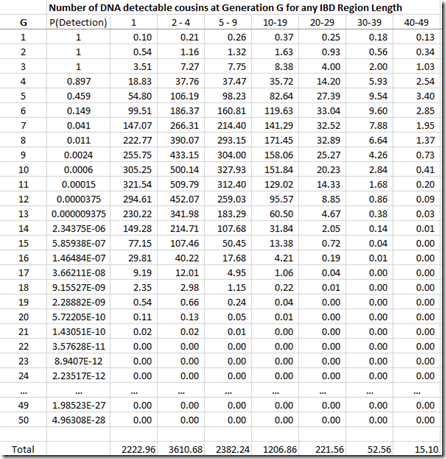
We’re not done yet. Once you get out to 3rd cousins and further, there is no longer a certainty that you will share any DNA with these relatives. You have to multiply every generation level by the probability that you will share at least some DNA. You can get that also from the ISOGG table I linked to above. The table can be extended at the end by dividing the probability by 4 for every additional generation. Then that probability is multiplied by the number of cousins (above) to give the expected number of detectable cousins, below:
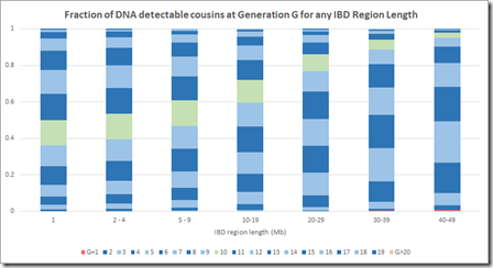
By dividing each column value by the column total, we can get the numbers needed that we can display in Speed and Balding format:
This is now a very different picture. Now most segments of any length come from a common ancestor 10 generations or less back. Even at the 1 Mb level, there are very few segments that come from further than 15 generations back.
This makes sense when you think about it, because segments 15 generations back have a miniscule chance of being shared between two people. In case of pileups coming from endogamy or a very distant prolific ancestor maybe 50 generations back (as in the Speed and Balding simulation) it’s very likely that there is a closer common relative somewhere in between that will be within 15 generations. Maybe Speed and Balding didn’t account for these when summarizing the simulation data – I don’t know.
Conclusion
I believe the above calculations and chart are correct using the Speed and Balding distribution data along with ISOGG’s generational data for the number of cousins and likelihood of DNA detection. It properly represents the DNA that you would match at different segment sizes for different generations.
Speed and Balding’s chart cannot be verified since they did not provide the details to do so, but inverting the distribution the way their simulation results might have been analyzed gives similar results to what they show.
I believe Speed and Balding’s chart greatly overestimates the number of generations that IBD segments came from. Their chart says that the >20 generation group makes up 50% of the IBD segments between 5 Mb and 10 Mb. Their >20 generation group remains a significant percentage of segments right up to 40 Mb segment length which I find very hard to believe, especially if we’re just talking about people who you match with.
Incorporating the likelihood of detecting DNA corrects what is not right with Speed and Balding’s Figure 2B and better represents the fraction of IBD DNA that can be expected to come from different generational levels in any Mb group.
All comments, criticisms and suggestions are welcome.
Figures 2Ab, 2B, Equation 5 and quote of text is reprinted by permission from Macmillan Publishers Ltd: Nature Reviews Genetics, Nature Publishing Group, Nov 18, 2014, copyright © 2014
—–
Followup: 10 days later (Nov 15), I have posted additional information in a new post: Another Estimate of Speed and Balding Figure 2B.
Update: Nov 16 – I made the correction pointed out by Andrew Millard on the ISOGG Facebook group, that it is the degree of cousinship on the ISOGG table I used, and the G should be 1 more than that number. I’ve updated all my tables and charts. The change it makes is small and does not change any of my observations or conclusion.
The ISOGG Facebook group is a closed group, but if you have been given access to it, the comments there about this article are a worthwhile read.





Joined: Mon, 13 Feb 2017
3 blog comments, 0 forum posts
Posted: Sun, 5 Nov 2017
Louis,
On an intuitive level, your analysis and conclusions have a ring of truth that I have found lacking in Speed and Baldwin. You present a much more encouraging picture for genetic genealogists!
Joined: Mon, 6 Nov 2017
2 blog comments, 0 forum posts
Posted: Mon, 6 Nov 2017
Louis, Thank you for this analysis and post - a tremendous service to the genetic genealogy community! We need someone like you with the math skills to help us understand and properly use the Speed and Balding paper. I had reluctantly accepted the way others had interpreted their widely seen Chart. But it just didn’t seem right to me. I have tried, in vain, to develop two different sets of curves. One I took a stab at in my segmentology blog - a distribution curve of IBD shared segments for each cousinship. It seems to me they would be centered around the calculated average value with longer and longer tails, which are needed to get cousins beyond 4th cousin to show up above 7cM. We have so many such distant cousins (as you pointed out in this blog), that some will be in the matching range. My second desired curve is a percent at each cousinship for our Matches - say 1% are 1C, 3% are 2C, 6% are 3C, 9% 4C, 12% 5C; 14% 6C; 16% 7C; 10% 8C; 5%9C; 4% 10C 2% for each of 11C-20C. Somewhere, the diminishing size of very distant cousin shared segment has to overtake the impact of the growing number of cousin. My gut estimate is that most of our Matches are in the 6-8 cousin range. Clearly this curve increases from very small number of very close cousins out to 4th cousin, but at some point a distribution curve has to peak and then fall - keeping the total under the curve at 100%. Two weeks ago, AncestryDNA had me at 50,000 Matches (probably over half are false), and 2,000 4C Matches (some probably 5C or 6C) - that would result in a flatter curve than my percents above..
Thanks again for your expertise and level headed reasoning about this topic. Jim
Joined: Tue, 7 Nov 2017
1 blog comment, 0 forum posts
Posted: Tue, 7 Nov 2017
Hi Louis, as my username probably gives away, I’m the first author of Speed and Balding (not to be confused with that terrible work from Speed and Baldwin infodoc rightly dismisses ;) ). I don’t follow the ISOOG blog, but a colleague alerted me to your blog post
Firstly, I’m incredibly flattered if it’s true that people have been using the figure we made. My research is mainly in common diseases, and particularly how we can use subtle similarities between very distantly related pairs of individuals to find genetic variants which increase / decrease risk of developing different conditions. Because I use very distantly related individuals, the similarity estimates are very small - between one pair it may be 0.001, between another -0.001. The tie in with the NRG paper you comment on, is that if I instead were to use more closely related individuals, the similarity values would increase, to the point they become recognisable as estimates of relatedness (ie 0.5 for full-siblings, 1 for twins). This poses an interesting problem, because when we examine distantly related individuals, there are 100s of different ways to measure similarity, each of which corresponds to a different assumption regarding how we believe causal variants affect risk for a particular trait (e.g., we might use one measure of similarity if studying type 2 diabetes, another for rheumatoid arthritis). Therefore, when people measure similarity between more closely related individuals, why do they tend to only use one or a few methods? Also, does our work on distantly related individuals provide an insight into which is the best method to use on more closely related individuals?
Hope some of that made a bit of sense. As for your article, it was very interesting to read your thoughts. Sorry that all the details are not clear in the paper - we thought there was a lot of important material to cover, but journal space is always at a premium, so I think we did very well to get as much as 10 pages. I really liked how you tied together the table and figure 2B, however, from my point of view, they were completely separate, except that I used the same mutation rates. Basically, for Figure 2b, I wrote a code (in the programming language C) which started with 10,000 individuals (5000 male, 5000 female). At each iteration, the code produced 10,000 children, each with a mum and a dad (while it’s standard convention to pick pairs at random, we modified this to reflect this is not how it works in the real world ;) ) Because it was a simulation, I could keep track of exactly what happened in each mating, i.e., which pieces of DNA a child got from their dad’s maternal DNA, and which from their dad’s paternal DNA, etc. I ended up with a long list of identity by descent (IBD) segments of varying length, allowing me to ask the question, if I observe a segment of length 10-20mb, what is the most likely G. One limitation is that the simulation is stochastic (lots of chance events) so I repeated it to check the results looked almost identical (i.e., the results were stable). A second is that we considered a finite number of generations (50) but I think I repeated with different numbers, again to check results were stable.
So it seems to me, your key point is that our figure exaggerates G for small chunks - for example, your results suggest that if we find two individuals share a segment 1-2MB long, they are more likely than not to have G<10, whereas our results suggeet the chance G<10 is about 20%. I am confident my simulations were reasonable and I think our estimates tied in with other results in the paper (but it’s been a few years so it’s not fresh in my mind). In response to one of your points, I am fairly confident my simulation kept track of the first most recent common ancestor (this was fairly easy to do, simply by recording each basepair of each of the 10,000 individuals as a number between 1 and 20,000 which indicates from which of the parental haplotypes it came, then it is straightforward to compute fraction IBD <=G generations (ie what fraction of the genome two individuals have inherited from a common ancestor no more than G generations ago), and in turn the fraction IBD exactly G generations (by subtracting the fraction <=G-1 from the fraction <=G). Therefore, I think the differences come from us asking slightly different questions rather than an error in either mine or your calculations (and yours may well be a more relevant question to ask). Hope this explanation helps in working out what this difference is!
Cheers, Doug
Joined: Sun, 9 Mar 2003
291 blog comments, 245 forum posts
Posted: Wed, 8 Nov 2017
Jim,
Thank you very much for your assessment. I too think that most of my segment matches (the ones that are valid) between 5 and 20 cM must be between 6 and 12 generations back since I have yet to identify any of them. But that’s what endogamy with just a 5 generation genealogy does.
I’m looking very forward to hearing your talks and meeting you in person in Houston this weekend at the FamilyTree DNA’s Genetic Genealogy Conference.
Louis
Joined: Sun, 9 Mar 2003
291 blog comments, 245 forum posts
Posted: Wed, 8 Nov 2017
Doug, (Professor Speed, Dr. Speed?)
Thank you for your thorough response to my post. If I understand your explanation correctly, you are doing everything exactly the way it should be done. The one thing you don’t mention is anything about filtering for only people who would show up in a person’s DNA match list. And that makes sense because you are studying diseases, not DNA relatives.
DNA testing companies filter the matches to only include people with a minimal total cM match and a minimum largest cM match. I describe this in my article. This filtering eliminates small individual segments coming from distant generations. Applying this filter to your results is the difference and converts your distribution for all segments with any match to an appropriate distribution for the matching segments of only the people in one’s match list.
I must encourage readers to view your presentation at WDYTYA Live from 8 Apr 2016.
Louis
Joined: Wed, 27 Sep 2017
6 blog comments, 0 forum posts
Posted: Wed, 8 Nov 2017
Louis
It makes no difference whether one is studying diseases or detecting DNA relatives. It’s still necessary to identify related people in the database.
The reason the testing companies filter small segments under 6 cMs or 7 cMs is not to exclude small segments from distant generations but for the very practical reason that these small segments cannot be accurately measured with genotype data and with the current IBD detection methods. An additional problem is that all the companies, with the exception of AncestryDNA, are giving us unphased matches. Without phasing there is a high false positive rate when reporting segments under 15 cMs. Even with phasing there are many false positives for small segments. See the 2014 article by Durand et al:
https://www.ncbi.nlm.nih.gov/pubmed/24784137
With computer simulations, as Doug has stated above, it’s possible to trace all segments, however small, because that can be controlled within the simulation.
The step you are proposing is therefore completely unnecessary which is why your figures differ so much from Speed and Balding’s. If you wish to translate the chart into data supplied by the companies all you have to do is ignore the data for the smaller segments that aren’t reported by the companies.
The point that both you and Jim seem to be missing is the fact that segments can date back a very long way. The distribution curve doesn’t end 10 generations ago. As Speed and Balding have shown, segments can trace back for 50 generations, and sometimes this includes very large segments. The number of our ancestors and the number of our cousins doubles every generation so we have many millions more cousins who share ancestors with us between 10 and 50 generations ago than we do cousins from the last 10 generations. Even though we are unlikely to match one specific cousin that long ago the fact that there are so many means that these are the cousins that dominate our match lists.
Speed and Balding’s simulations are backed up the informal research published by the geneticist Steve Mount in his blog post on “Genetic genealogy and the single segment”:
http://ongenetics.blogspot.co.uk/2011/02/genetic-genealogy-and-single-segment.html
It is also backed up by empirical data from the Ralph and Coop paper on “The geography of recent ancestry across Europe”:
http://journals.plos.org/plosbiology/article?id=10.1371/journal.pbio.1001555
See in particular this quote from the discussion:
“A related but far more intractable problem is to make a good guess of how long ago a certain shared genetic common ancestor lived, as personal genome services would like to do, for instance: if you and I share a 10 cM block of genome IBD, when did our most recent common ancestor likely live? Since the mean length of an IBD block inherited from five generations ago is 10 cM, we might expect the average age of the ancestor of a 10 cM block to be from around five generations. However, a direct calculation from our results says that the typical age of a 10 cM block shared by two individuals from the United Kingdom is between 32 and 52 generations (depending on the inferred distribution used). This discrepancy results from the fact that you are a priori much more likely to share a common genetic ancestor further in the past, and this acts to skew our answers away from the naive expectation—even though it is unlikely that a 10 cM block is inherited from a particular shared ancestor from 40 generations ago, there are a great number of such older shared ancestors.”
Ralph and Coop also have some very useful FAQs that explain some of these difficult concepts:
https://gcbias.org/european-genealogy-faq/
Joined: Wed, 27 Sep 2017
6 blog comments, 0 forum posts
Posted: Wed, 8 Nov 2017
Can I also suggest that people have a read of the comments in the ISOGG group on Facebook in the discussion about this blog post.
https://www.facebook.com/groups/isogg/permalink/10156092253692922/
In particular I recommend reading the comments from Dr Andrew Millard from the University of Durham. He has a background in mathematics and Bayesian analysis and has a good understanding of the issues.
Joined: Sun, 9 Mar 2003
291 blog comments, 245 forum posts
Posted: Wed, 8 Nov 2017
Thank you Debbie for your analysis, but I’m still not convinced.
You were correct on Facebook to say that the match filter would not affect results above 9 cM. So there must be some other reason why Speed and Balding give a greater than 20% chance that shared segments from 30 Mb to 40 Mb are from > 20 generations back.
Then it struck me that their simulation started with 10,000 founders, limited the population to approximately that size, and continued on for 50 generations. It starts out with non-related people having children together, but as the generations continue, with random pairings, it won’t be long until parents start to become related. It is likely in that model by 12 generations, almost every parent is related. By 20 generations they are likely all related in every way imaginable. What may be happening in the model is extreme endogamy for 50 full generations without any external DNA being added to the pot. We all know what happens in endogamy. Segments passed down multiple ways on multiple lines. This could very well be the reason for the expanded G values in their simulation. No external DNA added for 50 generations. If their simulation was a billion people growing to 7 billion people after 50 generations, I am fairly certain it would have given much different results, with much lower G values.
So therefore I do believe that my statistical model is a better one for the real world than Speed and Balding’s constrained simulation. And my final chart in Figure 2B format is a more realistic one for DNA testers.
With regards to Ralph and Coop, well that’s a completely different matter for another discussion since they don’t make sense to me at all. They say the mean length of a segment inherited from five generations is 10 cM. Using Equation 5 from Speed and Balding gives 7.8 Mb which is the same (since 3400 cM equal 2667 Mb). From 32 generations ago, Equation 5 gives 1.3 Mb and from 52 generations ago it is 0.8 Mb. So given that the average length of an IBD segment from 32 to 52 generations ago is between 0.8 and 1.3 Mb, how can the typical age of a 10 cM block be 32 to 52 generations??
Joined: Wed, 27 Sep 2017
6 blog comments, 0 forum posts
Posted: Thu, 9 Nov 2017
If you have a stable population over 50 generations then you do get extreme pedigree collapse. This is pretty much what has happened throughout human history with the exception of the last 300 years: https://en.wikipedia.org/wiki/World_population_estimates All humans are highly endogamous. It’s just a question of degree. After 50 generations each one of the 10,000 people in the simulation in the most recent generation would have a quadrillion genealogical ancestors which is clearly impossible because we know that the founding population was only 10,000 people. What happens is that people always marry someone to whom they are already related multiple times over. There are also simulations on this website that you might find of interest: http://burtleburtle.net/bob/future/ancestors.html The author provides a useful table showing the predicted number of genealogical and genetic ancestors at each generation. Like Speed and Balding he finds that it’s still possible to have genetic ancestors tracing back much further than people intuitively realise.
I don’t believe it makes sense to apply the Speed and Balding equation as far back as 32 generations. From what I understand this type of calculation assumes that our ancestors double with each generation when in reality the population just collapses upon itself and everyone is related. That is also why Ralph and Coop are seeing 10 cM segments going back such a long way. All Europeans are related to each other in multiple ways within the last 1000 years.
Joined: Sun, 9 Mar 2003
291 blog comments, 245 forum posts
Posted: Thu, 9 Nov 2017
Thanks, Debbie. I am now working with the help of your thoughts as well as those of Andrew Millard to try to statistically represent what Speed and Balding have simulated so as to better understand what their results represent. The constrained population is one thing (similar to a small version of Iceland over the past 50 generations or 1250 years). Also, since they go down to tiny amounts of DNA in their result, they may be considering any amount to be detectable. I’m in brainstorming mode and it may take me a few days to come up with something, especially since I’m now on my way to Houston for FTDNA’s annual Conference.
Joined: Fri, 6 Apr 2018
2 blog comments, 0 forum posts
Posted: Fri, 6 Apr 2018
You have been dancing around the phrase “conditional probability”, which is the big distinction between looking at data before and after the filter is applied. There is another conditional probability issue that arises because peoples match lists are sorted — regression to the mean, i.e., the regression effect.
When you look at list of matches, each has some DNA in common with you and each has some distance to a MRCA. The goal is to guess the latter based on the former. When correlation between two variables is strong the regression effect is minimal and the guesses should be pretty accurate. But lets ignore the matches with MRCA of, say, 4 or fewer generations back. The rest of the data is usually a huge list of weak matches, and the correlation between amount of DNA shared and generations to MRCA should be much weaker. Now when you sort this list of matches by shared DNA (still ignoring the strong matches) and just scroll through the beginning of that list, as most people probably do in practice, you are singling out among all of your weak matches those who have more shared DNA than most. And typically, the explanation for why these people would share more DNA than most of your weak matches is “luck”, rather than having a very close MRCA. What you should observe then is that the MRCAs with a lot of these “closer weak matches” is farther back than would be predicted by the regression model. I have found this anecdotally myself: for the handful of weak matches for whom we have traced a MRCA, the generational difference has usually been larger than had been predicted by the model. I am interested to know if other people have the same experience, since its impossible to tell here if the assumptions are in place for regression to the mean, or if so, how strong the effect should be.
Joined: Sun, 9 Mar 2003
291 blog comments, 245 forum posts
Posted: Sun, 8 Apr 2018
Barry:
You said: “for the handful of weak matches for whom we have traced a MRCA, the generational difference has usually been larger than had been predicted by the model”. I would expect that is because the one MRCA you identified is one of many MRCA’s that you and your match have. Neither of you has done enough research on your other lines to connect them to anyone else than the one MRCA you found. I am always aware of this being from an endogamous population.
And that one MRCA you found may be more distant than the other’s you have not found. In the end, the sum of the segments contributed by all the MRCA plus by-chance segments will bias the total cM to be higher than what you would expect for the one MRCA you found.
Louis
Joined: Fri, 6 Apr 2018
2 blog comments, 0 forum posts
Posted: Wed, 11 Apr 2018
The lack of information is possible, but I think unlikely. I have complete information back 5 generations, except for three ancestors who are all in Switzerland, and none of the three matches I am thinking of have anyone near Switzerland. At least two of my matches have similar completeness of records. So our predicted MRCAs of 4.2 and 4.8 generations back are definitely wrong.
There’s no way to rule out endogamy, as you say. But the point of my post is, attributing these issues to anything other than statistics is known as the “regression fallacy”. Yes, other factors may be contributing to regression toward the mean, but this effect will happen regardless. Everywhere I see discussion of endogamy, incomplete information, etc, but regression to the mean could play as big a role as these other factors and I never see it discussed.