Raw Data Comparison: FamilyTreeDNA vs MyHeritage DNA - Tue, 28 Mar 2017
Before I leave DNA and get back to Behold for a few weeks, I had one more set of results I wanted to report on.
A couple of weeks ago, I compared my MyHeritage DNA ethnicity results to my FamilyTreeDNA results, and also compared my match results.
There was one other comparison I had wanted to do. It’s to compare the Raw Data files of the two companies. My questions are:
- How similar the raw data downloads are.
- Do the differences significantly affect match results.
- Do the crossover points of segment matches significantly change.
Downloading Your Raw DNA Data
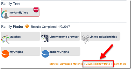
To download your raw data from FamilyTreeDNA, go to your Dashboard and click on “Download Raw Data”
On the next screen, select “Build 37 Raw Data Concatenated”
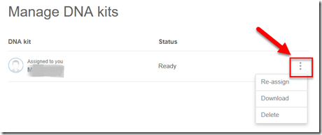
At MyHeritage DNA, it is not quite as obvious. Originally, I couldn’t find it and assumed you couldn’t download your data there, until I was shown how. What you do is go to your Manage DNA kits page, click on those 3 dots on the right, and select Download.
Comparing the Raw Data Files
The two companies, FamilyTreeDNA and MyHeritage both use the same DNA testing company Gene by Gene, Ltd. in Houston, Texas. In fact, Gene by Gene is the parent company of FamilyTreeDNA. MyHeritage chose Gene by Gene to be their lab, and Gene by Gene accepted the offer even though you could imagine MyHeritage DNA to be a competitor to Gene by Gene’s FamilyTreeDNA. I’m sure Gene by Gene must have thought it better to get MyHeritage’s lab business than to let them go off to some other lab. Even if this was a financially-based arrangement, it’s still nice to see a little bit of cooperation here between genealogy companies, just like it is to see FamilySearch’s partnership with MyHeritage and Ancestry and FindMyPast to share resources.
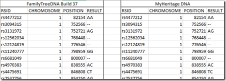
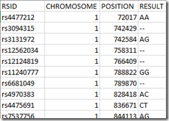
Given that it is the same lab doing the test, one would naturally expect the the lab results to be quite similar. I downloaded my two datasets and put them in one spreadsheet to compare them. They had exactly the same format. Here’s the first few lines of the two files side by side:
Think of RSID as the name of a particular position on a chromosome. The Position is in base-pair (bp) units from the beginning of the chromosome and is the information that Double Match Triangulator shows in its output. The result is one of the allele’s (A, C, G or T) from each parent at that location.
The data from the two companies both had 702,442 lines for chromosomes 1 through 22 with identical RSID, Chromosome and Position, and the entries of those were in the same order in each file, ordered not by RSID, but by Position. Having the first three fields matching exactly is a very good thing. They indicate that these download files of MyHeritage and FamilyTreeDNA are both using the same RSID definitions which are defined in what’s called a “Build”. FamilyTreeDNA allows you to download Build 36 or Build 37. MyHeritage only allows the download of Build 37, so I’m comparing Build 37 here.
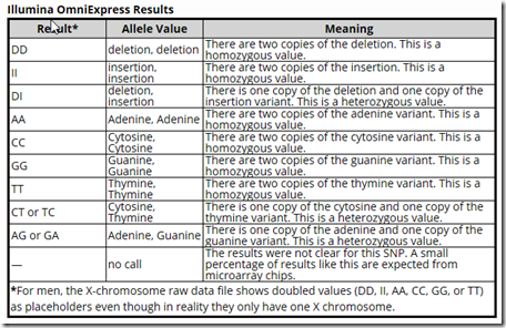
FamilyTree DNA gives a FAQ page: How do I read my Family Finder raw data file? In that FAQ they give the following useful table for interpreting the results:
I’m not sure why the table only lists two of the heterozygous values. There are 4 more: AC or CA, AT or TA, CG or GA, and GT or TG as you’ll see in the tables I created below. There were no insertion or deletion values in either of the downloads.
Comparing Autosomal Chromosomes 1 to 22
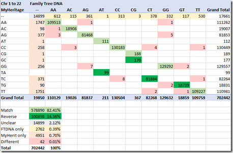
Comparing the Results field for those 702,442 values on chromosomes 1 to 22 gives for me the following counts:
578,890 (82.41%) of the entries (light green) match exactly.
FamilyTreeDNA does a nice thing and in their download shows the allele values of each pair in order alphabetically. So it only lists CT and not TC, only AG and not GA.
MyHeritage is not so nice. They show some of the pairs in the other order, with the higher alphabetical allele listed first. They do this for GC, TA, TC and TG (counts shown in dark green). And they show GC both ways, also as CG, and TA both ways, also as AT. Doing this makes me worry that there may be some third party tools that assume the order of alleles is one way or the other. If they do, they could present erroneous results from MyHeritage’s raw data. 100,898 (14.36%) of MyHeritage’s allele pairs match FamilyTree but are shown in the opposite order.
The FamilyTreeDNA table from their FAQ says that the double dash “—“ represents results that were not clear. They say this happens for a small percentage of the microchips. Well, 17,661 (2.5%) of the MyHeritage results are “unclear”, and 19,850 (2.8%) of the FamilyTreeDNA results are “unclear”. Of these, both companies agree that 14,899 (2.12%) of the pairs are “unclear”. At least they agree on most of them.
So up to now, we have 82.41% + 14.36% + 2.12% = 98.89% of the allele pairs matching between the two sets of raw data. That means we have a little over 1% that do not match. We are seeing what is the error rate between two different samples from the same person that are analyzed by the same lab. I don’t know the technical details as to how the companies determine the raw data from the samples, so I can’t speculate as to the reasons for the differences.
Breaking down the differences:
For 2,762 (0.39%), FamilyTreeDNA found a pair, but MyHeritage was unclear.
For 4,951 (0.70%), MyHeritage found a pair, but FamilyTreeDNA was unclear.
For 42 (0.01%), both companies found a pair, but the pair differed.
Build 36 versus Build 37
FamilyTreeDNA currently uses Build 36, not Build 37 when matching segments between people.As Gerrit van der Ende wrote: “A Build is a Genome assembly. As more is learned about the human genome, new Genome assemblies are released.”
The Chromosome Browser at FamilyTreeDNA, and the Chromosome Browser Results file you download from FamilyTreeDNA has positions based on Build 36. Build 36 had a few more RSIDs (702,457 for chromosomes 1 to 22 versus 702,442 for Build 37). There were 15 RSIDs deleted. Here is the beginning of my Build 36 download from FamilyTreeDNA:
Compare this to the Build 37 at the beginning of this article. The RSIDs are the same and the Results are the same, but all the Positions are different. The positions are not important for matching. Only the order of the RSIDs and the Results are important for matching. There were only 100 or so RSIDs that had a slight order difference, so different builds can be relatively easily translated into each other and matched against each other. What will be different between Builds are the Positions of the matching segments and the size of the segments.
GEDmatch, like FamilyTreeDNA, uses Build 36 for its comparisons. But 23andMe uses Build 37. So you can’t compare exact positions in Double Match Triangulator that were computed for FamilyTreeDNA or GEDmatch files with those computed at 23andMe..
MyHeritage’s positions in its raw data are all matching FamilyTreeDNA’s positions from the latter’s Build 37 download, so MyHeritage’s raw data is Build 37. I will not be able to tell whether their matches are Build 37 until MyHeritage provides a segment match download or a utility like a chromosome browser that shows segment match results. However I would guess, since they are a new company, they would use Build 37 matches, making their Positions compatible with 23andMe.
FamilyTreeDNA and GEDmatch are sort of stuck. They put together a matching system based on Build 36 and they’d have to remap all the results if they went to Build 37 for their matching. It would change the positions, but likely not change the match results significantly. That’s a lot of work for little gain, so I can see their reluctance to make the change.
Comparing Build 36 to Build 37 gives almost all the mapping that is needed. If it becomes important in the future for Double Match Triangulator, I see that I’d be able to do the mapping and present FamilyTreeDNA, GEDmatch, MyHeritage and 23andMe results all with comparable Positions, either Build 36 or Build 37.
Comparing the X Chromosomes
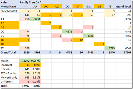
Doing the same comparison for the X chromosomes shows more differences between FamilyTreeDNA and MyHeritage DNA than chromosomes 1 to 22 did:
First of all, MyHeritage is missing 16 of the RSIDs that FamilyTreeDNA has. This wasn’t a problem for chromosomes 1 to 22 which matched exactly.
Then, if you look again at the FAQ above, you’ll see it says that for men who only have a single X chromosome, the one allele will be doubled, allowing only AA, CC, GG and TT. This is my raw data file, and I’m male. But the results show 46 combinations that include AC, AG, CT/TC and GT/TG. Those all have to be incorrect and I’ve marked them such.
And instead of only about 1% of the results where one company found a pair and the other was unclear, we are now up to over 5% of the X results being “unclear” for one of the companies, and another 641 or 4% being “unclear for both”. That means that about 9% of the X chromosome results are unknown or unagreed upon by the the test results that Gene by Gene produces from two DNA samples of the same person.
If 9% of the X chromosome results are missing or wrong, then for two people. 18% of the locations may be wrong between them. What effect might this have on X chromosome matching?
The Y chromosome
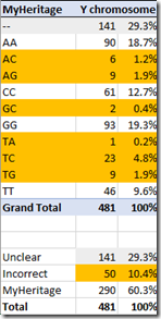
I was very surprised to see that the MyHeritage DNA raw data includes the Y chromosome. FamilyTreeDNA does not. So I can’t compare the two. All I can do is report on the Y results of MyHeritage DNA:
Again, there is only one Y chromosome, so according to the convention, the allele should be doubled. We see that only 60% of the 481 RSIDs have valid values of AA, CC, GG or TT.
Even without the FamilyTreeDNA raw data for the Y to compare with, the MyHeritage DNA raw data does not give much confidence regarding the accuracy of the Y chromosome interpretation as far as single allele processing goes. MyHeritage does not yet make report any results based on the Y chromosome, but they should double check this before they do.
Comparing Match Results at GEDmatch
The question now is whether these differences affect match results. One way to check this is to upload both files to GEDmatch.
Doing a One-to-one compare of the two files shows just 22 matches – one match for the length of each pair of chromosome. GEDmatch uses 3587.0 cM as the size of the 22 pairs, and that’s exactly what the One-to-one compare gives. GEDmatch must somehow filter out the 1% mismatches in its comparisons, which is good.
Comparing the 2 me’s to my uncle gives very close results. Out of 61 matching segment, one start location and one end location are a bit different. The total matches using the FamilyTreeDNA raw data is 2,006.4 cM and using the MyHeritage DNA data is 2,005.9 cM. Both give a largest segment of 88.3 cM.
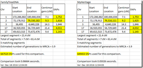
For a more distant relationship, such as my 3rd cousin, the results are almost the same with only a few small differences:
It does appear that even though there might be what appears to be a significant number of differences in the Raw Data files, they do not have a significant effect on the matches and only affect a few of the starting and ending locations, but not by much.
Checking out the X Chromosome and spot checking a few of my closest X matches, the results are similarly close, and X matching is not significantly affected.
Comparing Match Results at FamilyTreeDNA
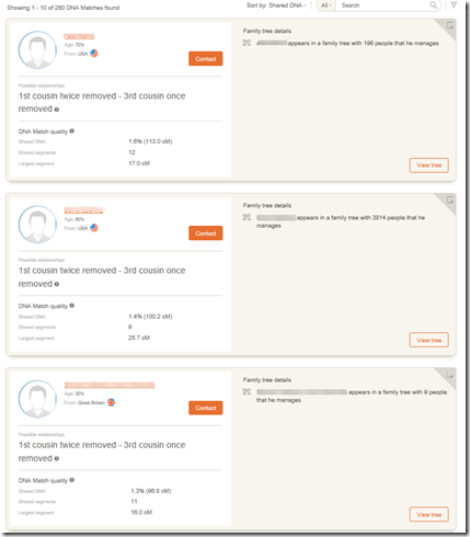
As a double check, I uploaded the MyHeritage DNA raw data into an account at FamilyTreeDNA. My original FamilyTreeDNA test give me 9860 matches. The MyHeritage raw data gives me 9724 matches.
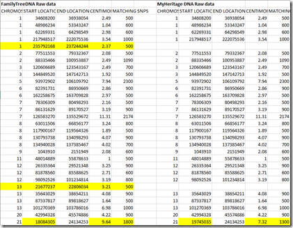
Of those, the cM total matches changed for 3717 of them, but the largest change was only 7.9 cM with the FamilyTreeDNA raw data giving a match of 107.1 cM and the MyHeritage DNA raw data giving a match of 99.2 cM. For this extreme case person, here is the comparison:
FamilyTreeDNA includes 2 segments of 2.37 cM and 3.21 cM that MyHeritage doesn’t, and one segment has a different start location. So even in this extreme case, the differences are not major.
Only 114 of the longest segments of the matches were different, with the largest difference being 3.6 cM that reduced a 16.4 cM longest segment down to 12.8 cM.
Again, this confirms that the differences in the Raw Data files do not have much of an affect on the match results.
Conclusions
- Comparing the raw data from FamilyTreeDNA and MyHeritage shows that for Chromosomes 1 to 22, there is disagreement or the result is unclear for 1.5% of the RSIDs. On the X chromosome, that percentage rises to 9%. On the Y chromosome, the percentage rises to 40%.
- These differences do not seem to have a significant effect on match results.
- A small number of start and end locations of segment matches may be different. This is worthy to note when I start getting Double Match Triangulator to analyze crossover points, but likely wont cause problems.
The raw data is more different than I expected it to be, but I’m very happy that it will make little difference to the match results.
—–
Update: Sept 28, 2017:
Raw Data Transfer
I was curious what raw data each company changes when you transfer the raw data from one to the other.
First I compared the MyHeritage transfer to FamilyTreeDNA with the original MyHeritage raw data.
The result is good. All FamilyTreeDNA changed in the raw data transferred from MyHeritage were the allele values GC, TA, TC and TG to CG, AT, CT and GT so that they would be in alphabetical order.
Unfortunately, I could not test the FamilyTreeDNA transfer to MyHeritage, because MyHeritage does not let you download the raw data of a transfer.





 Feedspot 100 Best Genealogy Blogs