Login to participate
  
Register   Lost ID/password?

Louis Kessler’s Behold Blog

Ancestry’s Timber Algorithm is Better Than You Think - Thu, 29 Oct 2020

Ancestry has recently made changes to its display of the amount of DNA you match with someone. The amount is shown in cM (centimorgans). Most DNA testers using their DNA for genealogy purposes know what cM are and what they represent.

image

Your DNA match list shows the Shared DNA you have with each of your matches.

The change Ancestry made that I’d like to talk about is the addition of “Unweighted shared DNA”. When you click on the “Shared DNA” link, you’ll be shown information containing this unweighted segment value:

image

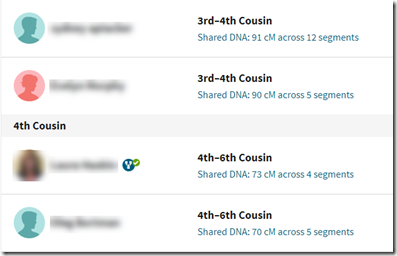
Here you’ll see a “Shared DNA” value of 91 cM and an “Unweighted shared DNA’” value also of 91 cM.  When the shared DNA value is 90 cM or more, the unshared value is always the same.

But when the shared DNA value is less than 90 cM, then the unweighted value can be more, and usually is.  The unweighted value can be as high as 89 cM.

image

Ancestry uses what they call their Timber algorithm to filter out pieces of DNA that it figures should not be considered when deciding if two people are related.

A lot of people, including myself, have been critical of Timber believing it removes segments that it shouldn’t and they were very happy with the new information that now shows the pre-Timber amount. You can’t easily get this amount for all your matches. You do have to click through each match one by one to get that match’s unweighted value. You cannot see them all on your DNA Matches page like you can the post-Timber values.


Comparing Average Shared Values

The research work I’m currently doing on one branch of my wife’s family with her cousin Terry Lasky includes some lines where we do not know if the ancestors are brother, half-brothers or first cousins. We have descendants of two ancestors who DNA tested that we can compare.  Those who are 3 generations down would be 3rd cousins if the ancestors are brothers, half 3rd cousins if they are half-brothers, and 4th cousins if the ancestors are 1st cousins. 

All of our family includes endogamy. Terry and I have been worried about the effect of endogamy on our cM shared values, and on the effect that the Ancestry Timber algorithm would have on our cM values.

Terry has 32 DNA testers from this branch who tested at Ancestry. Among the testers he had 138 pairs of them where he knew for sure how they were related and did not know of a second way they might be related, other than through endogamy.

Parent/child are 1 generation apart. At Ancestry DNA, parent/child pairs match with 3476 cM. Children are two generations apart (up to parent, down to other child). Their average match at Ancestry DNA should be 3/4 of a parent/child match or 2607 cM.  An uncle/aunt/nephew/niece is 3 generations apart, and an average match at Ancestry DNA in theory should average half of a parent/child match and be 1738 cM. From there on, every extra generation halves the cM matching. What we are doing is counting meiosis which is the number of times the cells recombine. Meiosis 6 for example can be 2nd cousins, 1st cousins twice removed, half 1st cousins once removed, or great-great-great-great grandparent/child and many other relationships. But they all should have the same theoretical average cM at Ancestry DNA and that should be 217 cM.

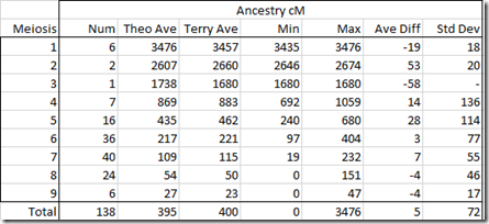
So what I did is averaged Terry’s known pairs by meiosis and compared them to what the theoretical average cM should be at Ancestry. It resulted in this table:

image

This very much surprised me when I first saw it. I had thought that Terry’s Ancestry numbers would be considerably higher than the theoretical averages due to endogamy. But Terry’s pairs averaged only 5 cM higher than the theoretical values. That is extremely close.

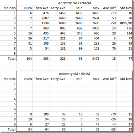
I scratched my head wondering why. These are the post-Timber values which had some segments removed by TImber. I decided to separate out the Timber affected numbers from those unaffected and divided the above table into >= 90 cM and < 90 cM.

image

Again I was surprised. The meiosis 7 and 8 have average differences of +29 and +76 for >= 90 cM.  They have average differences of -70 and -26 for < 90 cM.

It seems Ancestry optimized their 90 cM cutoff for Timber to get the averages in the meiosis levels to be close to the theoretical. What this seems to show is that it is not a good idea to separate out the two or to try to correct for their Timber algorithm.  Their numbers with Timber seem to be best.

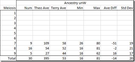
Just to check, I averaged out the Ancestry unweighted values for Terry’s pairs:

image

Meiosis 8 corrected is okay, but meiosis 7 has and average difference of -51.  Compare that to an average difference of 7 in the original raw values with Timber.  So I wouldn’t want to use these unweighted. Using Ancestry’s values with Timber seems best.

It seems that the Ancestry genetic scientists knew what they were doing with Timber. They seemed to have optimized it so that each meiosis level will average out very close to it’s theoretical value.


Blaine’s Shared cM Version 4.0

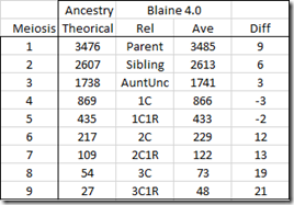
Well that was really good to know. Now I wanted to know how much Blaine Bettinger’s Shared cM Project v4 varied from the Ancestry theoretical averages. Surely Blaine’s would be different. His numbers were based on submissions of people who got cM values not just from Ancestry, but also from 23andMe, Family Tree DNA, GEDmatch, MyHeritage and others. Not all companies report exactly the same way. Family Tree DNA includes small segments down to 1 cM and will usually report higher shared cMs for the same two people. 

So here was a second surprise:

image

Blaine’s values are actually very close to the Ancestry theoretical value for the closer relationships.  Even meiosis 6 to 9 isn’t that far away. I attribute the slightly larger differences for the more distant relationships being due to some reported pairs being related an additional way that is adding to the amount. It isn’t much, just 12 to 21 cM,

None-the-less, Blaine’s numbers match up well with the Ancestry theoretical and that’s good to know.


Conclusion

Ancestry did Timber for a reason. It seems to me that they may have calibrated TImber so that the average cM for a given relationship would be the same as the theoretical average. Even if they didn’t do that calibration on purpose, it sure worked out well.

My recommendation is to use the Timber-based numbers, especially when comparing to Blaine’s shared cM project.

Don’t worry about the new unweighted Shared DNA values, and stop complaining so much about Timber.

Using WATO for Unknown Ancestral Relationships - Mon, 26 Oct 2020

Big update Oct 27:  Much easier way to do this than in my post below.  Leah Larkin informed me that I can do all 3 scenarios at once like this:
image

So all three hypothesis indeed can be included at once.

And the results with WATO Version 2 come out as:
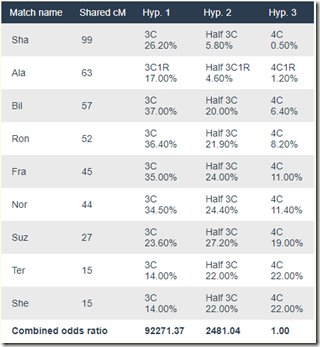
image

Showing Hypothesis 1 (Brother) is 37 times more likely than Hypothesis 2 (Half-Brother) which is 2481 times more likely than Hypothesis 3 (1st Cousin).

Much simpler! Many thanks to Leah and Andrew Millard on the WATO Facebook group for letting me see the light. 

I’ll leave my post below to show my original thinking.


Original Post:

In yesterday’s post, I wanted to see if the What Are The Odds (WATO) tool at the DNA Painter site would work for endogamy, and I came out satisfied that it does, for either Ancestry DNA numbers or Family Tree DNA numbers, with the < 7 cM matches removed from the latter.

WATO is designed to help you have a DNA match with someone where you don’t know for sure how that person is related to you. You build your tree in the WATO tool and add positions where you think your match might be. You set those positions to be Hypothesis.

Well, I’ve got a slightly different problem. We’ve got a bunch of DNA matches and I know where the fit in the tree.  What I don’t know is how the people at the top of the tree are related.

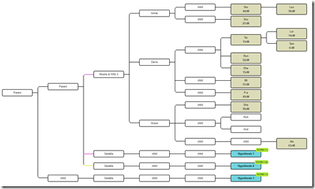
Let me start with the tree that I used as an example yesterday:
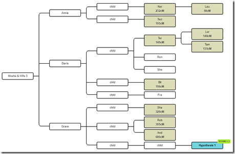
image

So these are all the relevant descendants of Moshe. The DNA testers are shown shaded. The Hypothesis 1 is a known tester who we simply used as a hypothesis.

Now there happens to have been a man named Gedalia who has the same last name as Moshe and came from the same town in Ukraine. We know of a few of Gedalia’s descendants who DNA tested and they are matches to the descendants of Moshe. What we don’t know and want to figure out is the relationship between Moshe and Gedalia. Could they be brothers? Half-brothers? First cousins?


Are Moshe and Gedalia Brothers?

So what I’ll do is expand the tree. I’ll add Gedalia to the tree as a brother to Moshe. I’ll add the descendants and mark the one we will use in this example as the Hypothesis: Now I’ll enter the cM shared between this descendant of Gedalia and each of the testers under Moshe.  I’ll used filtered Family Tree DNA numbers since those worked best yesterday:
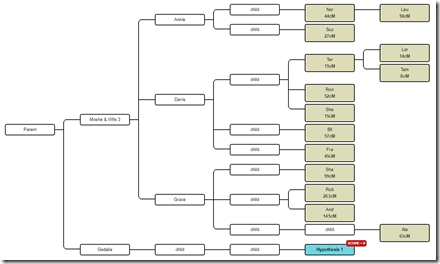
image

This gives us a score of zero, saying this is not possible.

So let’s take a look at the score calculation:
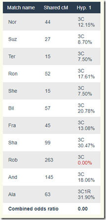
image

It’s saying that Rob is way too high at 263 cM to be a 3rd cousin.

But wait a minute! That is saying that Rob is related more closely than 3rd cousin to our Hypothesis person, who we’ll call: Hyp.  We know from the diagram above that through Moshe and Gedalia, he cannot be closer than 3rd cousins.  Since Rob’s cousin Sha and 1C1R Ala don’t have the same problem, they are okay. That must mean that Rob’s mother is related to Hyp, adding extra cMs to Rob and his sibling And. In fact, And is higher than all the rest at 145 cM, but not high enough to make being a 3rd cousin to Hyp an impossibility.

Since Rob and And are related another way to Hyp, what I’ll do is remove their shared DNA amounts from being included in the WATO calculations and run it again:
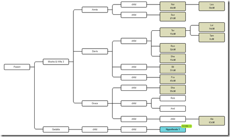
image

That’s better and now the Hypothesis shows up as possible. Here’s the score calculation:
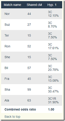
image

It’s the same as the above for the listed people, except that the Combined odds ratio is now 1.00.


Are Moshe and Gedalia Half-Brothers?

Let’s now do the same thing and just change Moshe and Gedalia to be half-brothers. WATO lets us do this and indicates they are halves with the coloured dotted lines to the left of their boxes:
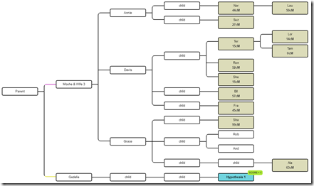
image

All of the scores have changed, but this scenario is still a possibility:
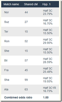
image


Are Moshe and Gedalia First Cousins?

Well, let’s delete Gedalia’s side and add him back in as a first cousin:
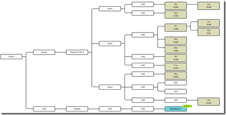
image

Once again, this is said to be possible. Here are the scores:
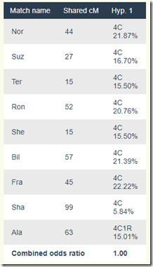
image


So Which Is More Likely? Brother? Half? Cousin?

WATO has a wonderful mechanism for comparing different Hypotheses. When you include more than one hypothesis in a scenario, it tells you which of the three is most likely and how many times more likely it is than the next. (See yesterday’s post for an example).

But here, I have three different trees each with only one Hypothesis. WATO won’t compare them for you.

Well I think I see what WATO is doing.  I may be wrong, but it looks like it is multiplying the probabilities together and comparing the results between the scenarios. So I can easily do that myself in a spreadsheet:
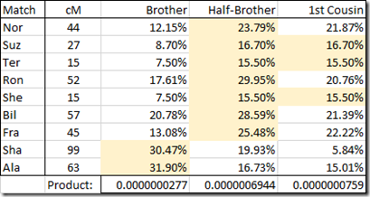
image

I have highlighted the most likely scenario for each match. Half-Brother wins this comparison with 7, versus 1st Cousin with 3 and Brother with just 2.

The line at the bottom contains the product of the 9 values above it. The highest value is Half-Brother which is 9 times larger, meaning it is 9 times more likely a possibility than 1st Cousin. 1st Cousin is 3 times more likely than Brother. And Brother is 25 times less likely than Half-Brother.

So there you have it. We haven’t proved anything, but at least we now know that all scenarios are possible and that half-brother is most likely.


Hint, Hint, Leah and Jonny

WATO is a wonderful tool to help you hypothesize where your DNA matches fit into your tree. That was what it was designed for.

But wouldn’t it be nice if WATO could also help you test different ancestral scenarios as well, as I have just done?  Well it can, if you follow the above procedure and do the comparison yourself,

WATO-Ancestors could be set up to make it easier for you by remembering the results of each of your scenarios, and then comparing them for you, so that you won’t have to yourself.


Update (80 minutes later): I didn’t realize when I was doing the analysis that I was using Version 1 of WATO. Version 2 includes new probability numbers taken from an update to Ancestry’s paper. See Leah’s article: Improving the Odds. The main improvement is that it now has much more detail for small matches.

You can switch from Version 1 to 2 very easily, so I did and I recalculated. Here’s the revised table:
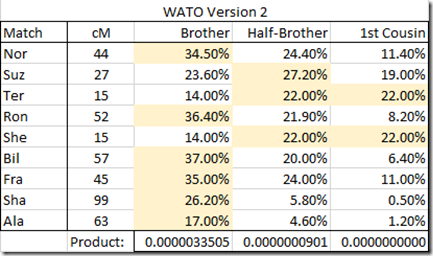
image

To tell the truth, it really changed the results. Now the conclusion is that Brother is the most likely relationship and that scenario is 37 times more likely than Half-Brother.

So make sure you use Version 2 of WATO to get the best probabilities.


Additional Idea: If you have more than one tester on the other side of the tree, you can calculate all the match values for each scenario for each of them, and then simply multiply out (or geometric mean) the “Product” line for each of them.

For example, in the above table, if I had a second person that gave Product numbers of 0.0000385 for Brother, 0.0000655 for Half-Brother and 0.0000073 for 1st Cousin, then

GMean(Brother) = (0.0000033505 * 0.0000385) ^ (1/2) = 0.0000114
GMean(Half-Brother) = (0.0000000901  * 0.000655) ^ (1/2) = 0.0000024
GMean(1st Cousin) = (0.0000000 * 0.0000073) ^ (1/2) = 0.0000000

If you don’t know what a geometric mean is, then just use a simple average which should still tell you which scenario is most likely.

Does WATO work well with Endogamous populations? - Sun, 25 Oct 2020

I’ve been quiet lately because I’ve been enjoying doing some research with my wife’s cousin Terry Lasky on one branch of their common families. Terry has got several dozen of his relatives on that side of the family to do DNA tests.

One aspect of what we are doing led to Jennifer Mendelsohn suggesting to me that we try WATO – the What Are the Odds tool built by Leah LaPerle Larkin and Jonny Perl.

I was concerned that the endogamy in our matches might add too much to the shared cM of two people. And I was also worried that the shared cM values that Family Tree DNA gives which are higher than the Ancestry DNA’s numbers would cause additional problems.

If WATO would not work for our known relationships, then we should not use it for our unknown relationships, meaning a test is required first.


Family Tree DNA data for a Known Relationship

So first step is to test WATO on a relationship which includes endogamy for a a person that has just one known pair of common ancestors with the other people. So there’s no other close multiple relationships that we know of other than the distant endogamy.

I took one of our starting ancestors, Moshe and Wife 3, who had three children. We have 14 DNA testers who between the children are 2C, 2C1R and 3C to each other. I took the 14th and made him the hypothesis and I created this with the WATO tool:

 WATO Tree for Endogamy(click on the image above to expand it)

So I created 11 hypothesis. 1, 2 and 3 are descendants of a child of Grace. 4, 5 and 6 are descendants of a child of Grace who is a half-sibling of Grace’s other children. 7, 8 and 9 are descendants of a full sibling of Grace, and 10 and 11 are descendants of a half sibling of Grace.

Each line of hypothesis is a half generation further away than the previous. And interestingly enough, the possible hypothesis marked in green move up a generation to compensate for this difference.

WATO’s gives you the calculated probabilities of each hypothesis:

image

So this is staying that Hypothesis 5, that this person is a child of a half-sibling of Grace’s other children is the most likely and is 52 times more likely than Hypothesis 2. Three other are possible and the rest are not statistically possible.

I love the detailed score calculation that Leah and Jonny put together. It gives you everything you’d ever want to know about each relationship in each hypothesis. And you can see how the probabilities were arrived at:

image

Now can you guess which Hypothesis is the correct one?  (spoiler below)


Family Tree DNA data stripping out small < 7 cM Matches

I had thought that WATO was based on the numbers from Blaine Bettinger’s Shared cM project. As I was calculating and writing the above, Jonny Perl responded to one of my posts on Facebook and said:

“The probabilities are actually separate from the shared cM project. In WATO v1 they’re from Ancestry’s white paper on matching and in v2 they are extrapolated from the probabilities AncestryDNA displays in the popup when you click on the cM amount.”

So I asked Jonny if it might be better to use Ancestry shared cM with WATO than to use Family Tree DNA data with it.  He said yes, and pointed me to his Individual Match Filter tool (IMF) to strip Family Tree DNA  matches back to a certain threshold (default is 7 cM).

Well Terry had done most of this work already for me and had many of the Family Tree DNA shared cM values already stripped back to only include 7 cM or larger values. I’m sure Terry would have liked to have known about Jonny’s tool as it would have saved him a lot of time.

I plotted Terry’s filtered numbers versus the non-filtered and got this relationship:

image

Notice this is a pretty strong relationship, and you can see that the trend line gives a pretty good estimate of what the filtered Family Tree DNA shared cM should be. The equation is basically saying that subtracting 50 cM from your unfiltered value will give you a decent filtered value. It should work okay for values greater than 100 cM, but obviously won’t be as good for smaller values.

Now I’ll use the filtered Family Tree DNA values in WATO instead of the unfiltered and we’ll see what happens:

WATO Tree for Endogamy (1)

This gives 5 feasible hypotheses with Hypothesis 2 coming on top being 8 times more likely than Hypothesis 5.

image


Ancestry DNA data for the same Known Relationship

Jonny’s comment also prompted me to try our Ancestry DNA matches. 11 of our 14 people above had originally tested at Ancestry DNA and those tests were later uploaded to FTDNA, so we still have 10 people we can compare with our 11th.

Putting in the Ancestry DNA shared cM values, we get this:

image

The Ancestry cM values we put in were actually not too different than the filtered FTDNA values. In fact, the biggest difference between them was 35 cM  The conclusion is the same with Hypothesis 2 being ahead of Hypothesis 5, but only being about 2 times more likely.

image


The Answer and Some Observations

The correct hypothesis is Hypothesis 2.

So it does seem that WATO is doing a good job and picked the correct Hypothesis with both the filtered FTDNA data and the Ancestry data.

Even though there are a few choices of possible valid Hypothesis, adding the known generational level of the tester and/or their age, will help to invalidate some and make one more likely.

I was worried that the endogamy would be a factor, but it seems not to be. Only the unfiltered FTDNA did not pick the correct answer on its number one hypothesis, and that is due to the many extra segments (about 50 cM worth) included in those numbers. As a result, it preferred to pick the hypothesis which was a half generation higher.

So this tells me that you needn’t worry about endogamy when using WATO. Just be sure to use either filtered FTDNA data (eliminating matches less than 7 cM) or use Ancestry DNA shared cM.